Bayesian optimization
![]()
Sources:
Introduction
Many optimization problems in machine learning are black box optimization problems where the objective function $f(\mathbf{x})$ is a black box function[1][2]. We do not have an analytical expression for $f$ nor do we know its derivatives. Evaluation of the function is restricted to sampling at a point $\mathbf{x}$ and getting a possibly noisy response.
If $f$ is cheap to evaluate we could sample at many points e.g. via grid search, random search or numeric gradient estimation. However, if function evaluation is expensive e.g. tuning hyperparameters of a deep neural network, probe drilling for oil at given geographic coordinates or evaluating the effectiveness of a drug candidate taken from a chemical search space then it is important to minimize the number of samples drawn from the black box function $f$.
This is the domain where Bayesian optimization techniques are most useful. They attempt to find the global optimimum in a minimum number of steps. Bayesian optimization incorporates prior belief about $f$ and updates the prior with samples drawn from $f$ to get a posterior that better approximates $f$. The model used for approximating the objective function is called surrogate model. Bayesian optimization also uses an acquisition function that directs sampling to areas where an improvement over the current best observation is likely.
Surrogate model
A popular surrogate model for Bayesian optimization are Gaussian processes (GPs). I wrote about Gaussian processes in a previous post. If you are not familiar with GPs I recommend reading it first. GPs define a prior over functions and we can use them to incorporate prior beliefs about the objective function (smoothness, ...). The GP posterior is cheap to evaluate and is used to propose points in the search space where sampling is likely to yield an improvement.
Acquisition functions
Proposing sampling points in the search space is done by acquisition functions. They trade off exploitation and exploration. Exploitation means sampling where the surrogate model predicts a high objective and exploration means sampling at locations where the prediction uncertainty is high. Both correspond to high acquisition function values and the goal is to maximize the acquisition function to determine the next sampling point.
More formally, the objective function $f$ will be sampled at $\mathbf{x}_t = \operatorname{argmax}_{\mathbf{x}} u(\mathbf{x} \lvert \mathcal{D}_{1:t-1})$ where $u$ is the acquisition function and $\mathcal{D}_{1:t-1} = \{(\mathbf{x}_1, y_1),...,(\mathbf{x}_{t-1}, y_{t-1})\}$ are the $t-1$ samples drawn from $f$ so far. Popular acquisition functions are maximum probability of improvement (MPI), expected improvement (EI) and upper confidence bound (UCB)[1]. In the following, we will use the expected improvement (EI) which is most widely used and described further below.
Optimization algorithm
The Bayesian optimization procedure is as follows. For $t = 1,2,...$ repeat:
- Find the next sampling point $\mathbf{x}_{t}$ by optimizing the acquisition function over the GP: $\mathbf{x}_t = \operatorname{argmax}_{\mathbf{x}} u(\mathbf{x} \lvert \mathcal{D}_{1:t-1})$
- Obtain a possibly noisy sample $y_t = f(\mathbf{x}_t) + \epsilon_t$ from the objective function $f$.
- Add the sample to previous samples $\mathcal{D}_{1:t} = \{\mathcal{D}_{1:t-1}, (\mathbf{x}_t,y_t)\}$ and update the GP.
Expected improvement
Expected improvement is defined as
$$\operatorname{EI}(\mathbf{x}) = \mathbb{E}\max(f(\mathbf{x}) - f(\mathbf{x}^+), 0)\tag{1}$$
where $f(\mathbf{x}^+)$ is the value of the best sample so far and $\mathbf{x}^+$ is the location of that sample i.e. $\mathbf{x}^+ = \operatorname{argmax}_{\mathbf{x}_i \in \mathbf{x}_{1:t}} f(\mathbf{x}_i)$.1 The expected improvement can be evaluated analytically under the GP model[3]:
$$ \operatorname{EI}(\mathbf{x}) = \begin{cases} (\mu(\mathbf{x}) - f(\mathbf{x}^+) - \xi)\Phi(Z) + \sigma(\mathbf{x})\phi(Z) &\text{if}\ \sigma(\mathbf{x}) > 0 \\ 0 & \text{if}\ \sigma(\mathbf{x}) = 0 \end{cases}\tag{2} $$
where
$$ Z = \begin{cases} \frac{\mu(\mathbf{x}) - f(\mathbf{x}^+) - \xi}{\sigma(\mathbf{x})} &\text{if}\ \sigma(\mathbf{x}) > 0 \\ 0 & \text{if}\ \sigma(\mathbf{x}) = 0 \end{cases} $$
where $\mu(\mathbf{x})$ and $\sigma(\mathbf{x})$ are the mean and the standard deviation of the GP posterior predictive at $\mathbf{x}$, respectively. $\Phi$ and $\phi$ are the CDF and PDF of the standard normal distribution, respectively. The first summation term in Equation (2) is the exploitation term and second summation term is the exploration term.
Parameter $\xi$ in Equation (2) determines the amount of exploration during optimization and higher $\xi$ values lead to more exploration. In other words, with increasing $\xi$ values, the importance of improvements predicted by the GP posterior mean $\mu(\mathbf{x})$ decreases relative to the importance of potential improvements in regions of high prediction uncertainty, represented by large $\sigma(\mathbf{x})$ values. A recommended default value for $\xi$ is $0.01$.
With this minimum of theory we can start implementing Bayesian optimization. The next section shows a basic implementation with plain NumPy and SciPy, later sections demonstrate how to use existing libraries. Finally, Bayesian optimization is used to tune the hyperparameters of a tree-based regression model.
Implementation with NumPy and SciPy
In this section, we will implement the acquisition function and its optimization in plain NumPy and SciPy and use scikit-learn for the Gaussian process implementation. Although we have an analytical expression of the optimization objective f in the following example, we treat is as black box and iteratively approximate it with a Gaussian process during Bayesian optimization. Furthermore, samples drawn from the objective function are noisy and the noise level is given by the noise variable. Optimization is done within given bounds. We also assume that there exist two initial samples in X_init and Y_init.
import numpy as np

%matplotlib inline

bounds = np.array([[-1.0, 2.0]])
noise = 0.2

def f(X, noise=noise):
    return -np.sin(3*X) - X**2 + 0.7*X + noise * np.random.randn(*X.shape)

X_init = np.array([[-0.9], [1.1]])
Y_init = f(X_init)
The following plot shows the noise-free objective function, the amount of noise by plotting a large number of samples and the two initial samples.
import matplotlib.pyplot as plt

# Dense grid of points within bounds
X = np.arange(bounds[:, 0], bounds[:, 1], 0.01).reshape(-1, 1)

# Noise-free objective function values at X
Y = f(X,0)

# Plot optimization objective with noise level
plt.plot(X, Y, 'y--', lw=2, label='Noise-free objective')
plt.plot(X, f(X), 'bx', lw=1, alpha=0.1, label='Noisy samples')
plt.plot(X_init, Y_init, 'kx', mew=3, label='Initial samples')
plt.legend();
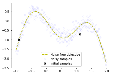
Goal is to find the global optimum on the left in a small number of steps. The next step is to implement the acquisition function defined in Equation (2) as expected_improvement function.
from scipy.stats import norm

def expected_improvement(X, X_sample, Y_sample, gpr, xi=0.01):
    '''
    Computes the EI at points X based on existing samples X_sample
    and Y_sample using a Gaussian process surrogate model.

    Args:
        X: Points at which EI shall be computed (m x d).
        X_sample: Sample locations (n x d).
        Y_sample: Sample values (n x 1).
        gpr: A GaussianProcessRegressor fitted to samples.
        xi: Exploitation-exploration trade-off parameter.

    Returns:
        Expected improvements at points X.
    '''
    mu, sigma = gpr.predict(X, return_std=True)
    mu_sample = gpr.predict(X_sample)

    sigma = sigma.reshape(-1, 1)

    # Needed for noise-based model,
    # otherwise use np.max(Y_sample).
    # See also section 2.4 in [1]
    mu_sample_opt = np.max(mu_sample)

    with np.errstate(divide='warn'):
        imp = mu - mu_sample_opt - xi
        Z = imp / sigma
        ei = imp * norm.cdf(Z) + sigma * norm.pdf(Z)
        ei[sigma == 0.0] = 0.0

    return ei
We also need a function that proposes the next sampling point by computing the location of the acquisition function maximum. Optimization is restarted n_restarts times to avoid local optima.
from scipy.optimize import minimize

def propose_location(acquisition, X_sample, Y_sample, gpr, bounds, n_restarts=25):
    '''
    Proposes the next sampling point by optimizing the acquisition function.

    Args:
        acquisition: Acquisition function.
        X_sample: Sample locations (n x d).
        Y_sample: Sample values (n x 1).
        gpr: A GaussianProcessRegressor fitted to samples.

    Returns:
        Location of the acquisition function maximum.
    '''
    dim = X_sample.shape[1]
    min_val = 1
    min_x = None

    def min_obj(X):
        # Minimization objective is the negative acquisition function
        return -acquisition(X.reshape(-1, dim), X_sample, Y_sample, gpr)

    # Find the best optimum by starting from n_restart different random points.
    for x0 in np.random.uniform(bounds[:, 0], bounds[:, 1], size=(n_restarts, dim)):
        res = minimize(min_obj, x0=x0, bounds=bounds, method='L-BFGS-B')
        if res.fun < min_val:
            min_val = res.fun[0]
            min_x = res.x

    return min_x.reshape(-1, 1)
Now we have all components needed to run Bayesian optimization with the algorithm outlined above. The Gaussian process in the following example is configured with a Matérn kernel which is a generalization of the squared exponential kernel or RBF kernel. The known noise level is configured with the alpha parameter.
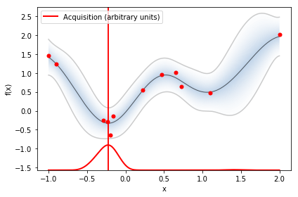
Bayesian optimization runs for 10 iterations. In each iteration, a row with two plots is produced. The left plot shows the noise-free objective function, the surrogate function which is the GP posterior predictive mean, the 95% confidence interval of the mean and the noisy samples obtained from the objective function so far. The right plot shows the acquisition function. The vertical dashed line in both plots shows the proposed sampling point for the next iteration which corresponds to the maximum of the acquisition function.
from sklearn.gaussian_process import GaussianProcessRegressor
from sklearn.gaussian_process.kernels import ConstantKernel, Matern
from bayesian_optimization_util import plot_approximation, plot_acquisition

# Gaussian process with Mat??rn kernel as surrogate model
m52 = ConstantKernel(1.0) * Matern(length_scale=1.0, nu=2.5)
gpr = GaussianProcessRegressor(kernel=m52, alpha=noise**2)

# Initialize samples
X_sample = X_init
Y_sample = Y_init

# Number of iterations
n_iter = 10

plt.figure(figsize=(12, n_iter * 3))
plt.subplots_adjust(hspace=0.4)

for i in range(n_iter):
    # Update Gaussian process with existing samples
    gpr.fit(X_sample, Y_sample)

    # Obtain next sampling point from the acquisition function (expected_improvement)
    X_next = propose_location(expected_improvement, X_sample, Y_sample, gpr, bounds)

    # Obtain next noisy sample from the objective function
    Y_next = f(X_next, noise)

    # Plot samples, surrogate function, noise-free objective and next sampling location
    plt.subplot(n_iter, 2, 2 * i + 1)
    plot_approximation(gpr, X, Y, X_sample, Y_sample, X_next, show_legend=i==0)
    plt.title(f'Iteration {i+1}')

    plt.subplot(n_iter, 2, 2 * i + 2)
    plot_acquisition(X, expected_improvement(X, X_sample, Y_sample, gpr), X_next, show_legend=i==0)

    # Add sample to previous samples
    X_sample = np.vstack((X_sample, X_next))
    Y_sample = np.vstack((Y_sample, Y_next))
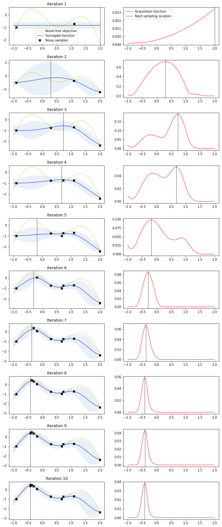
Note how the two initial samples initially drive search into the direction of the local maximum on the right side but exploration allows the algorithm to escape from that local optimum and find the global optimum on the left side. Also note how sampling point proposals often fall within regions of high uncertainty (exploration) and are not only driven by the highest surrogate function values (exploitation).
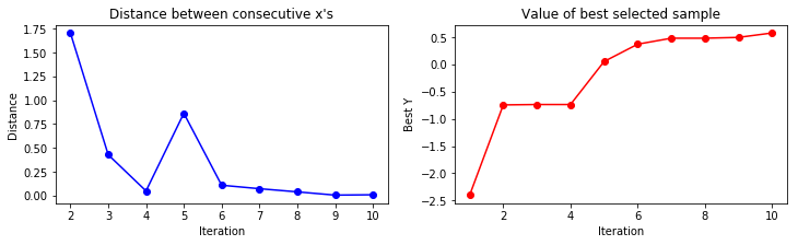
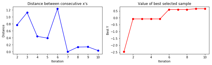
A convergence plot reveals how many iterations are needed the find a maximum and if the sampling point proposals stay around that maximum i.e. converge to small proposal differences between consecutive steps.
from bayesian_optimization_util import plot_convergence

plot_convergence(X_sample, Y_sample)
Bayesian optimization libraries
There are numerous Bayesian optimization libraries out there and giving a comprehensive overview is not the goal of this article. Instead, I'll pick two that I used in the past and show the minimum setup needed to get the previous example running.
Scikit-optimize
Scikit-optimize is a library for sequential model-based optimization that is based on scikit-learn. It also supports Bayesian optimization using Gaussian processes. The API is designed around minimization, hence, we have to provide negative objective function values. The results obtained here slightly differ from previous results because of non-deterministic optimization behavior and different noisy samples drawn from the objective function.
from sklearn.base import clone
from skopt import gp_minimize
from skopt.learning import GaussianProcessRegressor
from skopt.learning.gaussian_process.kernels import ConstantKernel, Matern
# Use custom kernel and estimator to match previous example
m52 = ConstantKernel(1.0) * Matern(length_scale=1.0, nu=2.5)
gpr = GaussianProcessRegressor(kernel=m52, alpha=noise**2)
r = gp_minimize(lambda x: -f(np.array(x))[0],
bounds.tolist(),
base_estimator=gpr,
acq_func='EI', # expected improvement
xi=0.01, # exploitation-exploration trade-off
n_calls=10, # number of iterations
n_random_starts=0, # initial samples are provided
x0=X_init.tolist(), # initial samples
y0=-Y_init.ravel())
# Fit GP model to samples for plotting results
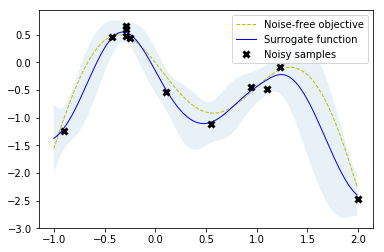
gpr.fit(r.x_iters, -r.func_vals)
# Plot the fitted model and the noisy samples
plot_approximation(gpr, X, Y, r.x_iters, -r.func_vals, show_legend=True)
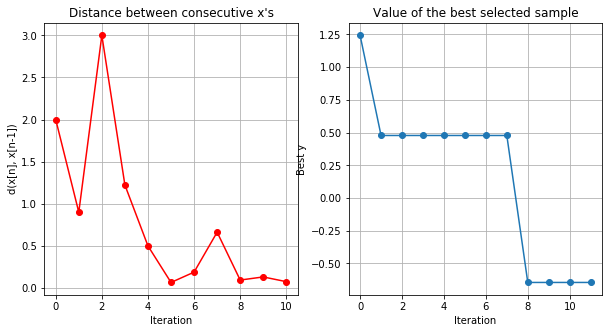
plot_convergence(np.array(r.x_iters), -r.func_vals)
GPyOpt
GPyOpt is a Bayesian optimization library based on GPy. The abstraction level of the API is comparable to that of scikit-optimize. The BayesianOptimization API provides a maximize parameter to configure whether the objective function shall be maximized or minimized (default). In version 1.2.1, this seems to be ignored when providing initial samples, so we have to negate their target values manually in the following example. Also, the built-in plot_acquisition and plot_convergence methods display the minimization result in any case. Again, the results obtained here slightly differ from previous results because of non-deterministic optimization behavior and different noisy samples drawn from the objective function.
import GPy
import GPyOpt

from GPyOpt.methods import BayesianOptimization

kernel = GPy.kern.Matern52(input_dim=1, variance=1.0, lengthscale=1.0)
bds = [{'name': 'X', 'type': 'continuous', 'domain': bounds.ravel()}]

optimizer = BayesianOptimization(f=f,
                                 domain=bds,
                                 model_type='GP',
                                 kernel=kernel,
                                 acquisition_type ='EI',
                                 acquisition_jitter = 0.01,
                                 X=X_init,
                                 Y=-Y_init,
                                 noise_var = noise**2,
                                 exact_feval=False,
                                 normalize_Y=False,
                                 maximize=True)

optimizer.run_optimization(max_iter=10)
optimizer.plot_acquisition()
optimizer.plot_convergence()
Application
This section demonstrates how to optimize the hyperparameters of an XGBRegressor with GPyOpt and how Bayesian optimization performance compares to random search. XGBRegressor is part of XGBoost, a flexible and scalable gradient boosting library. XGBRegressor implements the scikit-learn estimator API and can be applied to regression problems. Regression is performed on a small toy dataset that is part of scikit-learn.
from sklearn import datasets
from sklearn.model_selection import RandomizedSearchCV, cross_val_score

from scipy.stats import uniform
from xgboost import XGBRegressor

# Load the diabetes dataset (for regression)
X, Y = datasets.load_diabetes(return_X_y=True)

# Instantiate an XGBRegressor with default hyperparameter settings
xgb = XGBRegressor()

# and compute a baseline to beat with hyperparameter optimization
baseline = cross_val_score(xgb, X, Y, scoring='neg_mean_squared_error').mean()
Hyperparameter tuning with random search
For hyperparameter tuning with random search, we use RandomSearchCV of scikit-learn and compute a cross-validation score for each randomly selected point in hyperparameter space. Results will be discussed below.
# Hyperparameters to tune and their ranges
param_dist = {"learning_rate": uniform(0, 1),
              "gamma": uniform(0, 5),
              "max_depth": range(1,50),
              "n_estimators": range(1,300),
              "min_child_weight": range(1,10)}

rs = RandomizedSearchCV(xgb, param_distributions=param_dist,
                        scoring='neg_mean_squared_error', n_iter=25)

# Run random search for 25 iterations
rs.fit(X, Y);
Hyperparameter tuning with Bayesian optimization
To tune hyperparameters with Bayesian optimization we implement an objective function cv_score that takes hyperparameters as input and returns a cross-validation score. Here, we assume that cross-validation at a given point in hyperparameter space is deterministic and therefore set the exact_feval parameter of BayesianOptimization to True. Depending on model fitting and cross-validation details this might not be the case but we ignore that here.
bds = [{'name': 'learning_rate', 'type': 'continuous', 'domain': (0, 1)},
        {'name': 'gamma', 'type': 'continuous', 'domain': (0, 5)},
        {'name': 'max_depth', 'type': 'discrete', 'domain': (1, 50)},
        {'name': 'n_estimators', 'type': 'discrete', 'domain': (1, 300)},
        {'name': 'min_child_weight', 'type': 'discrete', 'domain': (1, 10)}]

# Optimization objective
def cv_score(parameters):
    parameters = parameters[0]
    score = cross_val_score(
                XGBRegressor(learning_rate=parameters[0],
                              gamma=int(parameters[1]),
                              max_depth=int(parameters[2]),
                              n_estimators=int(parameters[3]),
                              min_child_weight = parameters[4]),
                X, Y, scoring='neg_mean_squared_error').mean()
    score = np.array(score)
    return score

optimizer = BayesianOptimization(f=cv_score,
                                 domain=bds,
                                 model_type='GP',
                                 acquisition_type ='EI',
                                 acquisition_jitter = 0.05,
                                 exact_feval=True,
                                 maximize=True)

# Only 20 iterations because we have 5 initial random points
optimizer.run_optimization(max_iter=20)
Results
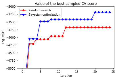
On average, Bayesian optimization finds a better optimium in a smaller number of steps than random search and beats the baseline in almost every run. This trend becomes even more prominent in higher-dimensional search spaces. Here, the search space is 5-dimensional which is rather low to substantially profit from Bayesian optimization. One advantage of random search is that it is trivial to parallelize. Parallelization of Bayesian optimization is much harder and subject to research (see [4], for example).
y_rs = np.maximum.accumulate(rs.cv_results_['mean_test_score'])
y_bo = np.maximum.accumulate(-optimizer.Y).ravel()

print(f'Baseline neg. MSE = {baseline:.2f}')
print(f'Random search neg. MSE = {y_rs[-1]:.2f}')
print(f'Bayesian optimization neg. MSE = {y_bo[-1]:.2f}')

plt.plot(y_rs, 'ro-', label='Random search')
plt.plot(y_bo, 'bo-', label='Bayesian optimization')
plt.xlabel('Iteration')
plt.ylabel('Neg. MSE')
plt.ylim(-5000, -3000)
plt.title('Value of the best sampled CV score');
plt.legend();
Baseline neg. MSE = -3498.95
Random search neg. MSE = -3678.77
Bayesian optimization neg. MSE = -3185.50
References
[1] Eric Brochu, Vlad M. Cora, Nando de Freitas, A Tutorial on Bayesian Optimization of Expensive Cost Functions.
[2] Jonas Mockus, Application of Bayesian approach to numerical methods of global and stochastic optimization.
[3] Donald R. JonesMatthias SchonlauWilliam J. Welch, Efficient Global Optimization of Expensive Black-Box Functions.
[4] Jialei Wang, Scott C. Clark, Eric Liu, Peter I. Frazier, Parallel Bayesian Global Optimization of Expensive Functions.
[5] Peter I. Frazier, A Tutorial on Bayesian Optimization.
-
This assumes noise-free observations. With noisy observations, $f(\mathbf{x}^+)$ is not directly available and is commonly replaced by the maximum of the GP posterior mean at the sample locations, $\mu^+ = \max_{\mathbf{x}_i \in \mathbf{x}_{1:t}} \mu(\mathbf{x}_i)$, a heuristic described in section 2.4 of [1] and used in the implementation below. Acquisition functions derived for noisy observations, such as the knowledge gradient[5], are beyond the scope of this article. ↩
Comments