Getting started with PyMC4
Bayesian neural networks
Sources:
Update: PyMC4 based on TensorFlow Probability will not be developed further. PyMC3 on Theano with the new JAX backend is the future.
This article demonstrates how to implement a simple Bayesian neural network for regression with an early PyMC4 development snapshot (from Jul 29, 2020). It can be installed with
pip install git+https://github.com/pymc-devs/pymc4@1c5e23825271fc2ff0c701b9224573212f56a534
I'll update this article from time to time to cover new features or to fix breaking API changes. The latest update (Aug. 19, 2020) includes the recently added support for variational inference (VI). The following sections assume that you have a basic familiarity with PyMC3. If this is not the case I recommend reading Getting started with PyMC3 first.
import logging
import pymc4 as pm
import numpy as np
import arviz as az

import tensorflow as tf
import tensorflow_probability as tfp
import matplotlib.pyplot as plt

%matplotlib inline

print(pm.__version__)
print(tf.__version__)
print(tfp.__version__)

# Mute Tensorflow warnings ...
logging.getLogger('tensorflow').setLevel(logging.ERROR)
4.0a2
2.4.0-dev20200818
0.12.0-dev20200818
Introduction to PyMC4
PyMC4 uses Tensorflow Probability (TFP) as backend and PyMC4 random variables are wrappers around TFP distributions. Models must be defined as generator functions, using a yield keyword for each random variable. PyMC4 uses coroutines to interact with the generator to get access to these variables. Depending on the context, PyMC4 may sample values from random variables, compute log probabilities of observed values, ... and so on. Details are covered in the PyMC4 design guide. Model generator functions must be decorated with @pm.model as shown in the following trivial example:
@pm.model
def model(x):
    # prior for the mean of a normal distribution
    loc = yield pm.Normal('loc', loc=0, scale=10)

    # likelihood of observed data
    obs = yield pm.Normal('obs', loc=loc, scale=1, observed=x)
This models normally distributed data centered at a location loc to be inferred. Inference can be started with pm.sample() which uses the No-U-Turn Sampler (NUTS). Samplers other than NUTS are currently not implemented in PyMC4.
# 30 data points normally distributed around 3
x = np.random.randn(30) + 3

# Inference
trace = pm.sample(model(x))
trace
arviz.InferenceData
- posterior
- sample_stats
- observed_data
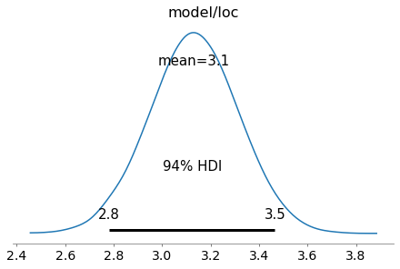
The returned trace object is an ArviZ InferenceData object. It contains posterior samples, observed data and sampler statistics. The posterior distribution over loc can be displayed with:
az.plot_posterior(trace, var_names=['model/loc']);
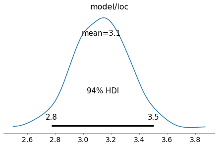
A recent addition to PyMC4 is variational inference and supported methods currently are advi and fullrank_advi. After fitting the model, posterior samples can be obtained from the resulting approximation object (representing a mean-field approximation in this case).
fit = pm.fit(model(x), num_steps=10000, method='advi')
trace = fit.approximation.sample(1000)
az.plot_posterior(trace, var_names=['model/loc']);
The history of the variational lower bound (= negative loss) during training can be displayed with
plt.plot(-fit.losses)
plt.ylabel('Variational lower bound')
plt.xlabel('Step');
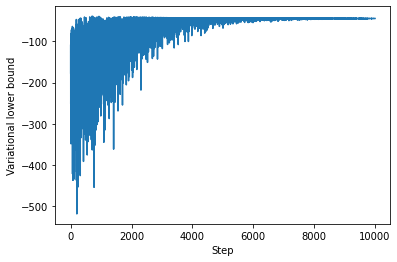
which confirms a good convergence after about 10,000 steps. Models can also be composed through nesting and used like other PyMC4 random variables.
@pm.model
def prior(name, loc=0, scale=10):
    loc = yield pm.Normal(name, loc=loc, scale=scale)
    return loc

@pm.model
def model(x):
    loc = yield prior('loc')
    obs = yield pm.Normal('obs', loc=loc, scale=1, observed=x)

trace = pm.sample(model(x))
az.plot_posterior(trace, var_names=['model/prior/loc']);
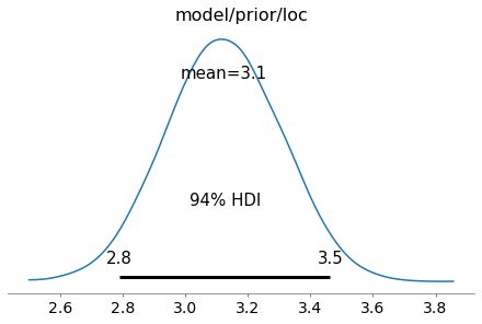
A more elaborate example is shown below where a neural network is composed of several layers.
Example dataset
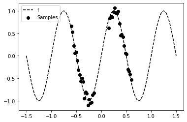
The dataset used in the following example contains N noisy samples from a sinusoidal function f in two distinct regions (x1 and x2).
def f(x, noise):
    """Generates noisy samples from a sinusoidal function at x."""
    return np.sin(2 * np.pi * x) + np.random.randn(*x.shape) * noise

N = 40
noise = 0.1

x1 = np.linspace(-0.6, -0.15, N // 2, dtype=np.float32)
x2 = np.linspace(0.15, 0.6, N // 2, dtype=np.float32)

x = np.concatenate([x1, x2]).reshape(-1, 1)
y = f(x, noise=noise)

x_test = np.linspace(-1.5, 1.5, 200, dtype=np.float32).reshape(-1, 1)
f_test = f(x_test, noise=0.0)

plt.scatter(x, y, marker='o', c='k', label='Samples')
plt.plot(x_test, f_test, 'k--', label='f')
plt.legend();
Bayesian neural network
Model definition
To model the non-linear relationship between x and y in the dataset we use a ReLU neural network with two hidden layers, 5 neurons each. The weights of the neural network are random variables instead of deterministic variables. This is what makes a neural network a Bayesian neural network. Here, we assume that the weights are independent random variables.
The neural network defines a prior over the mean loc of the data likelihood obs which is represented by a normal distribution. For simplicity, the aleatoric uncertainty (noise) in the data is assumed to be known. Thanks to PyMC4's model composition support, priors can be defined layer-wise using the layer generator function and composed to a neural network as shown in function model. During inference, a posterior distribution over the neural network weights is obtained.
@pm.model
def layer(name, x, n_in, n_out, prior_scale, activation=tf.identity):
    w = yield pm.Normal(name=f'{name}_w', loc=0, scale=prior_scale, batch_stack=(n_in, n_out))
    b = yield pm.Normal(name=f'{name}_b', loc=0, scale=prior_scale, batch_stack=(1, n_out))

    return activation(tf.tensordot(x, w, axes=[1, 0]) + b)

@pm.model
def model(x, y, prior_scale=1.0):
    o1 = yield layer('l1', x, n_in=1, n_out=5, prior_scale=prior_scale, activation=tf.nn.relu)
    o2 = yield layer('l2', o1, n_in=5, n_out=5, prior_scale=prior_scale, activation=tf.nn.relu)
    o3 = yield layer('l3', o2, n_in=5, n_out=1, prior_scale=prior_scale)

    yield pm.Normal(name='obs', loc=o3, scale=noise, observed=y)
The batch_stack parameter of random variable constructors is used to define the shape of the random variable.
Inference
Tensorflow will automatically run inference on a GPU if available. With the current version of PyMC4, MCMC inference using NUTS on a GPU is quite slow compared to a multi-core CPU (need to investigate that in more detail). To enforce inference on a CPU set environment variable CUDA_VISIBLE_DEVICES to an empty value. There is no progress bar visible yet during sampling but the following shouldn't take longer than a few minutes on a modern multi-core CPU.
# MCMC inference with NUTS
trace = pm.sample(model(x, y, prior_scale=3), burn_in=100, num_samples=1000)
Variational inference is significantly faster but the results are less convincing than the MCMC results. I need to investigate that further to see if I'm doing something wrong or if this is an issue with the current PyMC4 development snapshot. We'll therefore use the MCMC results in the following section. If you want to see the VI results, run the following cell instead of the previous one.
# Variational inference with full rank ADVI
fit = pm.fit(model(x, y, prior_scale=0.5), num_steps=150000, method='fullrank_advi')

# Draw samples from the resulting mean-field approximation
trace = fit.approximation.sample(1000)
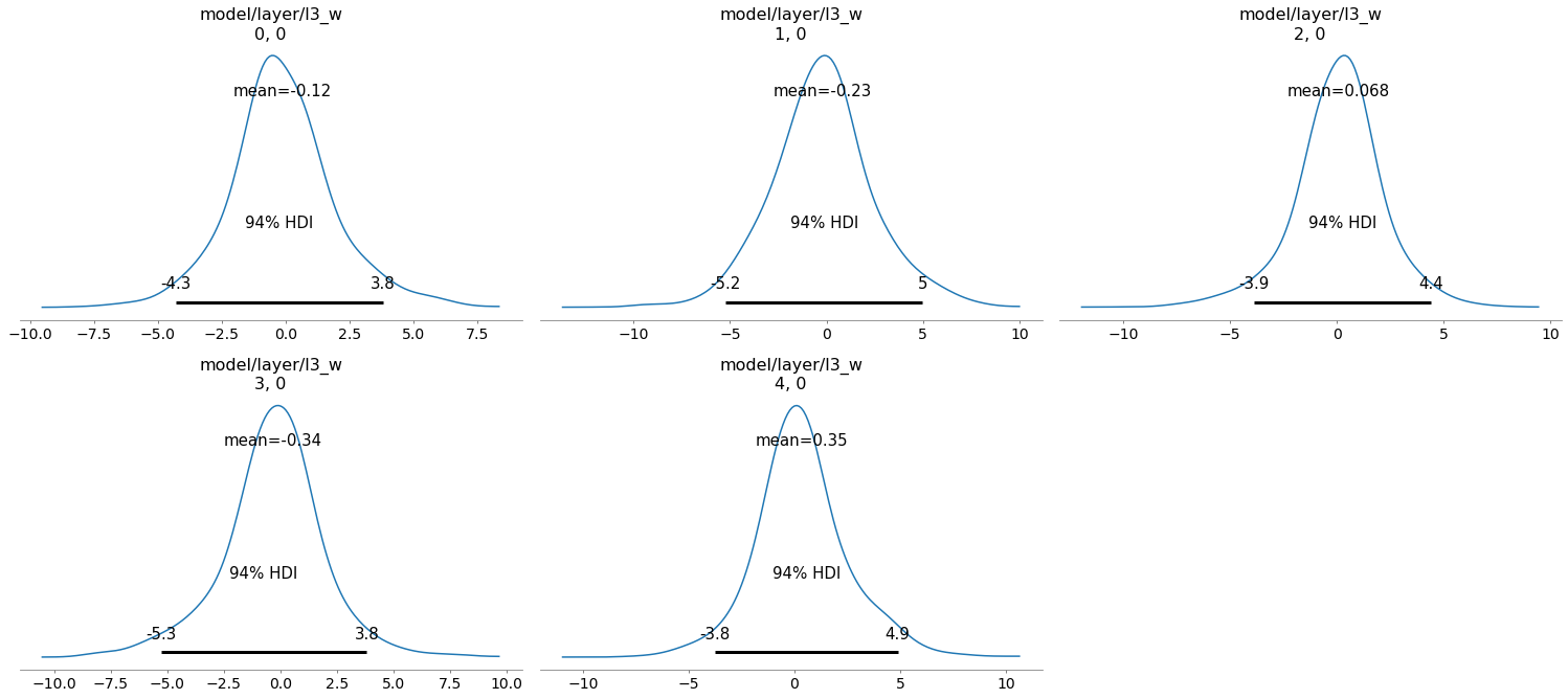
The full trace can be visualized with az.plot_trace(trace). Here, we only display the posterior over the last layer weights (without bias).
az.plot_posterior(trace, var_names="model/layer/l3_w");
Prediction
To obtain posterior predictive samples for a test set x_test we simply call the model generator function again with the test set as argument. This is a nice improvement over PyMC3 which required to setup a shared Theano variable for setting test set values. Target values are ignored during predictive sampling, only the shape of the target array y matters, hence we set it to an array of zeros with the same shape as x_test.
draws_posterior = pm.sample_posterior_predictive(model(x=x_test, y=np.zeros_like(x_test)), trace, inplace=False)
draws_posterior.posterior_predictive
<xarray.Dataset>
Dimensions:          (chain: 10, draw: 1000, model/obs_dim_0: 200, model/obs_dim_1: 1)
Coordinates:
  * chain            (chain) int64 0 1 2 3 4 5 6 7 8 9
  * draw             (draw) int64 0 1 2 3 4 5 6 ... 993 994 995 996 997 998 999
  * model/obs_dim_0  (model/obs_dim_0) int64 0 1 2 3 4 5 ... 195 196 197 198 199
  * model/obs_dim_1  (model/obs_dim_1) int64 0
Data variables:
    model/obs        (chain, draw, model/obs_dim_0, model/obs_dim_1) float32 ...
Attributes:
    created_at:     2020-08-19T12:12:02.008383
arviz_version: 0.9.0- chain: 10
- draw: 1000
- model/obs_dim_0: 200
- model/obs_dim_1: 1
- chain(chain)int640 1 2 3 4 5 6 7 8 9
array([0, 1, 2, 3, 4, 5, 6, 7, 8, 9])
- draw(draw)int640 1 2 3 4 5 ... 995 996 997 998 999
array([ 0, 1, 2, ..., 997, 998, 999])
- model/obs_dim_0(model/obs_dim_0)int640 1 2 3 4 5 ... 195 196 197 198 199
array([ 0, 1, 2, 3, 4, 5, 6, 7, 8, 9, 10, 11, 12, 13, 14, 15, 16, 17, 18, 19, 20, 21, 22, 23, 24, 25, 26, 27, 28, 29, 30, 31, 32, 33, 34, 35, 36, 37, 38, 39, 40, 41, 42, 43, 44, 45, 46, 47, 48, 49, 50, 51, 52, 53, 54, 55, 56, 57, 58, 59, 60, 61, 62, 63, 64, 65, 66, 67, 68, 69, 70, 71, 72, 73, 74, 75, 76, 77, 78, 79, 80, 81, 82, 83, 84, 85, 86, 87, 88, 89, 90, 91, 92, 93, 94, 95, 96, 97, 98, 99, 100, 101, 102, 103, 104, 105, 106, 107, 108, 109, 110, 111, 112, 113, 114, 115, 116, 117, 118, 119, 120, 121, 122, 123, 124, 125, 126, 127, 128, 129, 130, 131, 132, 133, 134, 135, 136, 137, 138, 139, 140, 141, 142, 143, 144, 145, 146, 147, 148, 149, 150, 151, 152, 153, 154, 155, 156, 157, 158, 159, 160, 161, 162, 163, 164, 165, 166, 167, 168, 169, 170, 171, 172, 173, 174, 175, 176, 177, 178, 179, 180, 181, 182, 183, 184, 185, 186, 187, 188, 189, 190, 191, 192, 193, 194, 195, 196, 197, 198, 199]) - model/obs_dim_1(model/obs_dim_1)int640
array([0])
- model/obs(chain, draw, model/obs_dim_0, model/obs_dim_1)float3226.57001 26.04135 ... -14.317561
array([[[[ 2.65700092e+01],
         [ 2.60413494e+01],
         [ 2.57281590e+01],
         ...,
         [-4.75241995e+00],
         [-4.78487253e+00],
         [-4.75552654e+00]],

        [[ 3.16064491e+01],
         [ 3.10987301e+01],
         [ 3.04416885e+01],
         ...,
         [-5.26556778e+00],
         [-5.20179415e+00],
         [-5.47270155e+00]],

        [[ 4.52943230e+01],
         [ 4.45980377e+01],
         [ 4.39933929e+01],
         ...,
...
         ...,
         [-5.59512615e+00],
         [-5.61213923e+00],
         [-5.73862267e+00]],

        [[ 2.81977844e+00],
         [ 2.81224990e+00],
         [ 3.02726460e+00],
         ...,
         [-5.47826385e+00],
         [-5.42433500e+00],
         [-5.45992947e+00]],

        [[ 3.89422917e+00],
         [ 3.80268312e+00],
         [ 3.86203289e+00],
         ...,
         [-1.39646444e+01],
         [-1.41936607e+01],
         [-1.43175611e+01]]]], dtype=float32)
- created_at :
- 2020-08-19T12:12:02.008383
- arviz_version :
- 0.9.0
The predictive mean and standard deviation can be obtained by averaging over chains (axis 0) and predictive samples (axis 1) for each of the 200 data points in x_test (axis 2).
predictive_samples = draws_posterior.posterior_predictive.data_vars['model/obs'].values

m = np.mean(predictive_samples, axis=(0, 1)).flatten()
s = np.std(predictive_samples, axis=(0, 1)).flatten()
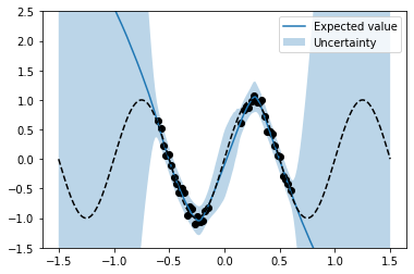
These statistics can be used to plot model predictions and their variances (together with function f and the noisy training data). One can clearly see a higher predictive variance (= higher uncertainty) in regions outside the training data.
plt.plot(x_test, m, label='Expected value');
plt.fill_between(x_test.flatten(), m + 2 * s, m - 2 * s, alpha = 0.3, label='Uncertainty')

plt.scatter(x, y, marker='o', c='k')
plt.plot(x_test, f_test, 'k--')

plt.ylim(-1.5, 2.5)
plt.legend();
If you think something can be improved in this article (and I'm sure it can) or if I missed other important aspects of PyMC4 please let me know.
Comments