A gentle introduction to Rotary Position Embedding
![]()
The Transformer model is invariant to reordering of the input sequence. For sequence modeling, position information must therefore be explicitly included. Rotary position embedding is an approach for including relative position information. It is a multiplicative approach, in contrast to most other approaches which are additive.
Position information basics
This article assumes that you have a basic understanding of the Transformer architecture and the scaled dot product attention mechanism. An excellent introduction is given here. To recap, self-attention first transforms token embeddings $\mathbf{x}_m$ and $\mathbf{x}_n$ at positions $m$ and $n$ to query $\mathbf{q}_m$, key $\mathbf{k}_n$ and value $\mathbf{v}_n$.
$$ \begin{align} \mathbf{q}_m &= f_q(\mathbf{x}_m, m) \\ \mathbf{k}_n &= f_k(\mathbf{x}_n, n) \\ \mathbf{v}_n &= f_v(\mathbf{x}_n, n) \end{align} \tag{1} $$
where $\mathbf{q}_m$, $\mathbf{k}_n$ and $\mathbf{v}_n$ have position information encoded through functions $f_q$, $f_k$ and $f_v$, respectively. The compatibility between tokens at positions $m$ and $n$ is given by an attention weight $\alpha_{m,n}$.
$$ \alpha_{m,n} = { {\exp(a_{m,n}) \over \sqrt{d}} \over {\sum_{j=0}^N {\exp(a_{m,j}) \over \sqrt{d}}}} \tag{2} $$
where $a_{m,n} = \mathbf{q}_m^\mathsf{T} \mathbf{k}_n$ are the elements of the attention matrix $\mathbf{A}$. The self-attention output $\mathbf{o}_m$ at position $m$ is a weighted sum over values $\mathbf{v}_n$.
$$ \mathbf{o}_m = \sum_{n=1}^N \alpha_{m,n} \mathbf{v}_n \tag{3} $$
Most approaches add position information to token representations i.e. use an addition operation to include absolute or relative position information. For example, for including absolute position information, a typical choice for Eq. $(1)$ is
$$ \begin{align} \mathbf{q}_m &= \mathbf{W}_q(\mathbf{x}_m + \mathbf{p}_m) \\ \mathbf{k}_n &= \mathbf{W}_k(\mathbf{x}_n + \mathbf{p}_n) \\ \mathbf{v}_n &= \mathbf{W}_v(\mathbf{x}_n + \mathbf{p}_n) \\ \end{align} \tag{4} $$
where $\mathbf{p}_m$ and $\mathbf{p}_n$ are representations of positions $m$ and $n$ that are either generated using a predefined function or learned*). $\mathbf{W}_q$, $\mathbf{W}_k$, and $\mathbf{W}_v$ are learned matrices for query, key and value projections, respectively.
Relative position information is often included by formulating $\mathbf{q}_m^\mathsf{T} \mathbf{k}_n$ with definitions from Eq. $(3)$ as
$$ \mathbf{q}_m^\mathsf{T} \mathbf{k}_n = \mathbf{x}_m^\mathsf{T} \mathbf{W}_q^\mathsf{T} \mathbf{W}_k \mathbf{x}_n + \mathbf{x}_m^\mathsf{T} \mathbf{W}_q^\mathsf{T} \mathbf{W}_k \mathbf{p}_n + \mathbf{p}_m^\mathsf{T} \mathbf{W}_q^\mathsf{T} \mathbf{W}_k \mathbf{x}_n + \mathbf{p}_m^\mathsf{T} \mathbf{W}_q^\mathsf{T} \mathbf{W}_k \mathbf{p}_n \tag{5} $$
and modifying the RHS of Eq. $(5)$ by replacing absolute position information $\mathbf{p}_m$ and $\mathbf{p}_n$ with relative position information, among other modifications. This adds relative position information to the attention matrix $\mathbf{A} = (a_{mn})$ only. Relative position information can also be added to values through an extension of Eq. $(3)$. See this overview for further details.
Rotary position embedding
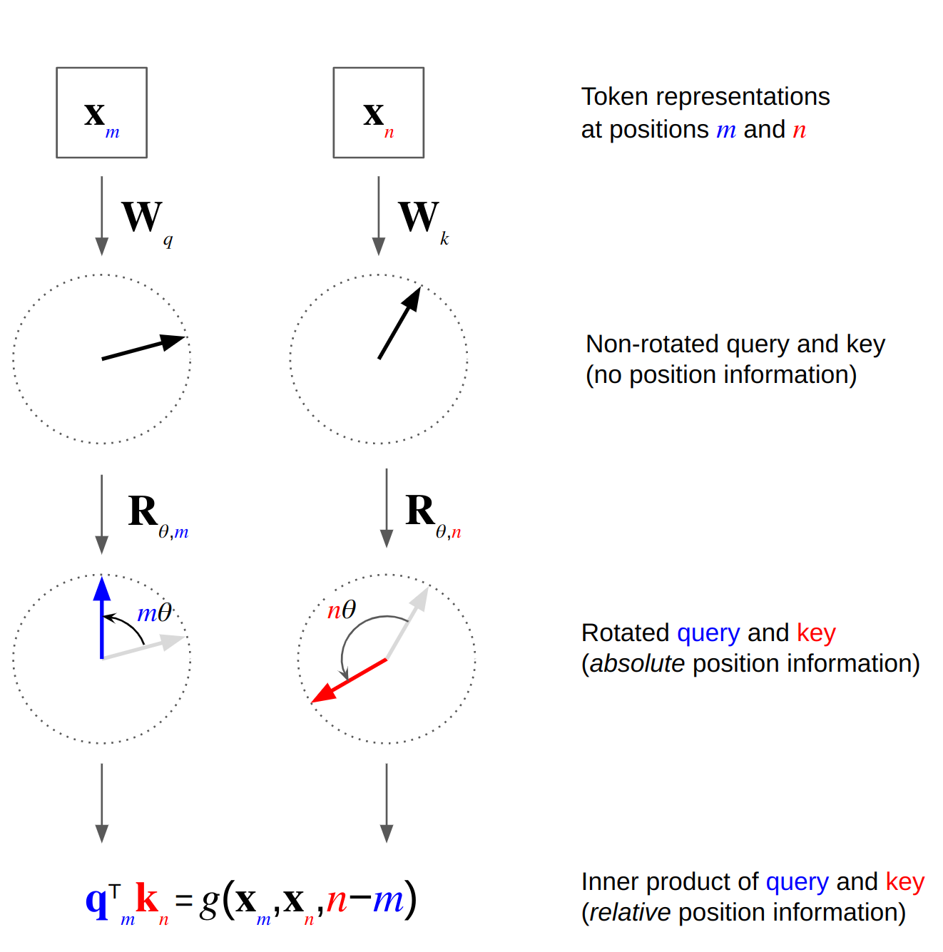
Rotary position embedding is an approach for including relative position information into the attention matrix, but it differs from other approaches that it first multiplies queries and keys with a rotation matrix i.e. it rotates $\mathbf{W}_q \mathbf{x}_m$ and $\mathbf{W}_k \mathbf{x}_n$ before taking their inner product. The rotation matrix is a function of absolute position. Calculating the inner products of rotated queries and keys results in an attention matrix that is a function of relative position information only. So how does this work?
More formally, we want the inner product of $f_q(\mathbf{x}_m, m)$ and $f_k(\mathbf{x}_n, n)$ to be a function $g$ that encodes position information only in the relative form:
$$ \langle f_q(\mathbf{x}_m, m), f_k(\mathbf{x}_n, n) \rangle = g(\mathbf{x}_m, \mathbf{x}_n, n-m) \tag{6} $$
As shown in the paper, a solution of Equation $(6)$ is given by the following definitions of $f_q$, $f_k$ and $g$:
$$ \begin{align} f_q(\mathbf{x}_m, m) &= \mathbf{R}_{\theta,m} \mathbf{W}_q \mathbf{x}_m = \mathbf{q}_m \\ f_k(\mathbf{x}_n, n) &= \mathbf{R}_{\theta,n} \mathbf{W}_k \mathbf{x}_n = \mathbf{k}_n \\ g(\mathbf{x}_m, \mathbf{x}_n, n-m) &= \mathbf{x}_m^\mathsf{T} \mathbf{W}_q^\mathsf{T} \mathbf{R}_{\theta,n-m} \mathbf{W}_k \mathbf{x}_n = \mathbf{q}_m^\mathsf{T} \mathbf{k}_n \end{align} \tag{7} $$
where
$$ \mathbf{R}_{\theta,n-m} = \mathbf{R}_{\theta,m}^\mathsf{T} \mathbf{R}_{\theta,n} \tag{8} $$
$\mathbf{R}_{\theta,t=\{m,n,n-m\}}$ is a rotation matrix. In 2D, $\mathbf{R}_{\theta,t}$ is defined as
$$ \mathbf{R}_{\theta,t} = \begin{pmatrix} \cos t\theta & -\sin t\theta \\ \sin t\theta & \cos t\theta \\ \end{pmatrix} \tag{9} $$
where $\theta$ is a non-zero constant. So the rotation of $f_q(\mathbf{x}_m, m)$ and $f_k(\mathbf{x}_n, n)$ by an angle that is a function of absolute position $m$ and $n$, respectively, results in an inner product $\mathbf{q}_m^\mathsf{T} \mathbf{k}_n$ that encodes relative position information $n - m$ only (see Fig. 1). Values do not encode position information i.e. $\mathbf{v}_n = \mathbf{W}_v\mathbf{x}_n$.
A generalization of the 2D rotation matrix to $d$-dimensional space is a block-diagonal matrix
$$ \mathbf{R}_{\Theta,t}^d = \begin{pmatrix} \cos t\theta_1 & -\sin t\theta_1 & 0 & 0 & \cdots & 0 & 0 \\ \sin t\theta_1 & \cos t\theta_1 & 0 & 0 & \cdots & 0 & 0 \\ 0 & 0 & \cos t\theta_2 & -\sin t\theta_2 & \cdots & 0 & 0 \\ 0 & 0 & \sin t\theta_2 & \cos t\theta_2 & \cdots & 0 & 0 \\ \vdots & \vdots & \vdots & \vdots & \ddots & \vdots & \vdots & \\ 0 & 0 & 0 & 0 & \cdots & \cos t\theta_{d/2} & -\sin t\theta_{d/2} \\ 0 & 0 & 0 & 0 & \cdots & \sin t\theta_{d/2} & \cos t\theta_{d/2} \\ \end{pmatrix} \tag{10} $$
that divides the space into $d/2$ subspaces, each using a different value of $\Theta = \\{\theta_i = 10000^{-2(i-1)/d},i \in [1,2,\dots,d/2]\\}$. For relative positions $t = n - m = 0$, $\mathbf{R}_{\Theta,t}^d$ is the identity matrix and hence
$$ \begin{align} f_q(\mathbf{x}_m, 0) &= \mathbf{W}_q \mathbf{x}_m \\ f_k(\mathbf{x}_n, 0) &= \mathbf{W}_q \mathbf{x}_n \\ g(\mathbf{x}_m, \mathbf{x}_n, 0) &= \mathbf{x}_m^\mathsf{T} \mathbf{W}_q^\mathsf{T}\mathbf{W}_k \mathbf{x}_n \\ \end{align} \tag{11} $$
Properties
The diagonal of the attention matrix $\mathbf{A}$, where $n - m = 0$, contains the inner products of non-rotated queries and keys and therefore doesn't encode relative position information. For off-diagonal elements, where $n - m \neq 0$, the inner product decays with increasing distance. A proof for an upper bound of the decay is given in section 3.4.3 of the rotary position encoding paper. This supports the intuition that tokens with larger distance have weaker connection than tokens with smaller distance.
Rotary position embedding is also compatible with linear self-attention which is a kernel-based method that avoids explicitly computing the attention matrix. Other approaches for relative position encoding that directly operate on the attention matrix can't therefore be used. Rotary position embedding on the other hand derives relative position information from rotated queries and keys alone without adding values to the attention matrix directly.
Another property of rotary position embedding is the flexibility to sequence length. Although not discussed in the paper I think it is because relative position information can be generated with a predefined function for any values of $m$ and $n$.
Implementation
import torch
from einops import rearrange, repeat
Multiplication with the sparse rotation matrix $\mathbf{R}_{\Theta,t}^d$ defined in Eq. $(10)$ is computationally inefficient. A more efficient realization is
$$ \mathbf{R}_{\Theta,t}^d \mathbf{u} = \begin{pmatrix} u_1 \\ u_2 \\ u_3 \\ u_4 \\ \vdots \\ u_{d-1} \\ u_d \end{pmatrix} \otimes \begin{pmatrix} \cos m\theta_1 \\ \cos t\theta_1 \\ \cos t\theta_2 \\ \cos t\theta_2 \\ \vdots \\ \cos t\theta_{d/2} \\ \cos t\theta_{d/2} \end{pmatrix} + \begin{pmatrix} -u_2 \\ u_1 \\ -u_4 \\ u_3 \\ \vdots \\ -u_d \\ u_{d-1} \end{pmatrix} \otimes \begin{pmatrix} \sin t\theta_1 \\ \sin t\theta_1 \\ \sin t\theta_2 \\ \sin t\theta_2 \\ \vdots \\ \sin t\theta_{d/2} \\ \sin t\theta_{d/2} \end{pmatrix} \tag{12} $$
where vector $\mathbf{u}$ is a query or a key. There are numerous implementations available for rotary position embedding. Examples of PyTorch implementations are here, here or here. They usually first encode absolute positions $t$ up to a maximum sequence length as multiples of inverse frequencies $\theta_1,\theta_2,\dots,\theta_{d/2}$, followed by duplicating each element along the frequency dimension.
def freq_pos_enc(dim, max_seq_len):
    # inverse frequencies [theta_1, theta_2, ..., theta_dim/2]
    inv_freq = 1.0 / (10000 ** (torch.arange(0, dim, 2, dtype=torch.float) / dim))  # (dim/2,)
    # positions up to max_seq_len
    pos = torch.arange(max_seq_len)  # (max_seq_len,)
    # frequency position encoding (outer product: pos x inv_freq)
    pos_enc = torch.einsum("p, f -> p f", pos, inv_freq)  # (max_seq_len, dim/2)
    # duplicate each element along inverse frequency dimension
    return repeat(pos_enc, "... f -> ... (f r)", r=2)  # (max_seq_len, dim)
This precomputes the $\sin$ and $\cos$ arguments in Equation $(12)$ and is called frequency position encoding here. For evaluating Equation $(12)$ a rotate_half helper that shuffles the elements of $\mathbf{u}$ in the second term of the addition is helpful.
def rotate_half(u):
    # last dimension of u is [u1, u2, u3, u4, ...]
    u = rearrange(u, '... (d r) -> ... d r', r=2)
    u1, u2 = u.unbind(dim=-1)
    u = torch.stack((-u2, u1), dim=-1)
    # last dimension of result is [-u2, u1, -u4, u3, ...]
    return rearrange(u, '... d r -> ... (d r)')
Rotation of $\mathbf{u}$, using a given frequency position encoding, can then be implemented as
def rotate(u, pos_enc):
    num_tokens = u.shape[-2]
    pos_enc = pos_enc[:num_tokens]
    return u * pos_enc.cos() + (rotate_half(u) * pos_enc.sin())
Here's a complete usage example. Starting from a batch of sequences of queries and keys (for all attention heads) they are first rotated before computing their inner product to obtain the attention matrix for each head and example in the batch.
batch_size = 2
num_heads = 8
seq_len = 64
head_dim = 32

# random queries and keys
q = torch.randn(batch_size, num_heads, seq_len, head_dim)
k = torch.randn(batch_size, num_heads, seq_len, head_dim)

# frequency-encode positions 1 - 512
pos_enc = freq_pos_enc(dim=head_dim, max_seq_len=512)

# encode absolute positions into queries and keys
q_rot = rotate(q, pos_enc)
k_rot = rotate(k, pos_enc)

# take inner product of queries and keys to obtain attention
# matrices that have relative position information encoded
attn = torch.einsum("b h i c, b h j c -> b h i j", q_rot, k_rot)
assert attn.shape == (batch_size, num_heads, seq_len, seq_len)
*) Regarding the difference between position embedding and position encoding, my understanding is that the term position encoding is used when position information is generated with a predefined function, e.g. a sinusoidal function, whereas position embedding is used when position information is learned. Although rotary position embedding uses a predefined function to generate position information it is yet called a position embedding approach by its authors.
Comments