Training compute-optimal Perceiver AR language models
Notebook and code for this article are available here.
Introduction
In Training Compute-Optimal Large Language Models [1] (the Chinchilla paper) the authors describe how to determine the optimal model size $N_{opt}$ and number of training tokens $D_{opt}$ for a given compute budget $C$, and how $N_{opt}$ and $D_{opt}$ scale with $C$. These scaling laws are applicable to decoder-only transformer language models.
In this article I describe how I applied these scaling laws to Perceiver AR [2] language models and discuss the experimental results. Perceiver AR is a simple extension to a decoder-only transformer, introducing cross-attention to a longer prefix sequence. I run Perceiver AR scaling experiments on small scale, for model sizes ranging from 17M to 108M parameters, but the very same approach can also be used at larger scale.
Scaling laws
The Chinchilla paper [1] assumes a power law relationship between compute $C$ and compute-optimal model size $N_{opt}$ and number of training tokens $D_{opt}$.
$$ \begin{align} N_{opt} &\propto C^a \\ D_{opt} &\propto C^b \end{align} \tag{1} $$
The authors use three different approaches to determine exponents $a$ and $b$, and obtain similar results. For approach 1 $a=0.50$ and $b=0.50$, for approach 2 $a = 0.49$, $b = 0.51$. I skip approach 3 as it is not used in this article.
This suggest that the number of model parameters and number of training tokens should be scaled more or less equally with compute $C$. For actually calculating $N_{opt}$ and $D_{opt}$ from $C$ we still need the factors of proportionality $k_N$ and $k_D$:
$$ \begin{align} N_{opt} &= k_N C^a \\ D_{opt} &= k_D C^b \end{align} \tag{2} $$
The paper doesn't provide these factors directly, but they can be derived from estimates of $N_{opt}$ and $D_{opt}$ for different compute budgets $C$. These estimates are provided in Tables 3 and A3 in [1]. By fitting $(2)$ to these estimates
import pandas as pd

from scaling.laws import fit_scaling_law

# Estimates from Table 3 in [1]
df_1 = pd.read_csv("data/estimates/approach_1.csv")
# Estimates from Table A3 in [1]
df_2 = pd.read_csv("data/estimates/approach_2.csv")

scaling_law_1 = fit_scaling_law(df_1["FLOPs"], df_1["Parameters"], df_1["Tokens"], a=0.50, b=0.50)
scaling_law_2 = fit_scaling_law(df_2["FLOPs"], df_2["Parameters"], df_2["Tokens"], a=0.49, b=0.51)
we obtain
print(scaling_law_1)
N_opt = 0.0877 * C ** 0.50
D_opt = 1.8960 * C ** 0.50
for approach 1 and
print(scaling_law_2)
N_opt = 0.1448 * C ** 0.49
D_opt = 1.1519 * C ** 0.51
for approach 2.
Perceiver AR
Perceiver AR is a simple extension of a plain decoder-only transformer such as GPT-2, for example. A core building block of both is the decoder layer consisting of a self-attention layer followed by a position-wise MLP. Self-attention uses a causal attention mask.
Perceiver AR additionally cross-attends to a longer prefix of the input sequence in its first attention layer. This layer is a hybrid self- and cross-attention layer. Self-attention is over the last n positions of the input sequence, with a causal attention mask, cross-attention is from the last $n$ positions to the first $m$ positions. The length of the input sequence is $m + n$. This allows a Perceiver AR to process a much larger context than decoder-only transformers which are based on self-attention only.
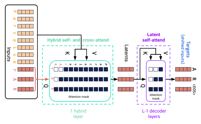
The output of the hybrid attention layer are $n$ latent arrays corresponding to the last $n$ tokens of the input sequence. These are further processed by a stack of $L - 1$ decoder layers where the total number of attention layers is $L$. A final layer (not shown in Fig. 1) predicts the target token for each latent position. The weights of the final layer are shared with the input embedding layer.
Except for the initial cross-attention to the prefix sequence, a Perceiver AR is architecturally identical to a decoder-only transformer. In the following, I refer to this part of Perceiver AR as the self-attention part and to the last n tokens of the input sequence as latent tokens.
The self-attention part includes input and position embedding of latent tokens, self-attention followed by a position-wise MLP in the hybrid layer and all decoder layers, and target token prediction in the final output layer. The remaining cross-attention part includes input and position embedding of the prefix tokens and cross-attention from latent positions to prefix positions.
Compute estimates
For estimating the FLOPs required to train Perceiver AR models I'm using the compute estimates from Table 1 in [3] and additionally include the estimates for the embedding layer and the final output layer as done in Appendix F of [1]. This is implemented in class ComputeEstimator. Update: FLOPs computation as described in Appendix F of [1] seems to be incorrect. You can find all details here and how it affects the results in this article (TL;DR the conclusion remains valid).
The training FLOPs per latent token for the self-attention part of Perceiver AR can be estimated with the self_attn() method. The training FLOPs per latent token for the initial cross-attention can be estimated with cross_attn(). An example:
from scaling.flops import ComputeEstimator

ce = ComputeEstimator(vocab_size=32000, max_seq_len=2048, num_latents=512)

num_channels = 512
num_layers = 9

c_self = ce.self_attn(num_channels, num_layers)
print(f"Self-attention training FLOPs per latent token: {c_self:.2e}")

c_cross = ce.cross_attn(num_channels, prefix_dropout=0.5)
print(f"Cross-attention training FLOPs per latent token: {c_cross:.2e}")

cross_fraction = c_cross / (c_cross + c_self)
print(f"Cross-attention contribution to overall compute: {cross_fraction * 100:.2f}%")
Self-attention training FLOPs per latent token: 2.82e+08
Cross-attention training FLOPs per latent token: 7.10e+06
Cross-attention contribution to overall compute: 2.45%
The self_attn() method can also be used for estimating the training FLOPs of plain decoder-only transformer models. The results from this method are very close to the common $C \approx 6N$ approximation where $N$ is the number of model parameters including embedding weights.
from scaling.flops import num_self_attn_params

n_self = num_self_attn_params(
    num_channels=num_channels,
    num_layers=num_layers,
    num_latents=ce.num_latents,
    num_prefix=ce.num_prefix,
    vocab_size=ce.vocab_size,
)

# Simple approximation of training FLOPs (per latent token)
c_self_approx = 6 * n_self

print(f"C_self / C_self_approx = {c_self / c_self_approx:.2f}")
C_self / C_self_approx = 1.05
The scaling laws in [1] have been derived from training decoder-only transformers, hence, they can only be applied to the self-attention part of Perceiver AR. For calculating $N_{opt}$, we must therefore use the estimated training FLOPs of the self-attention part.
The cross-attention part requires extra compute. Its contribution to the overall compute increases with prefix sequence length and decreases with the number of decoder layers i.e. model size. It makes up only a few percent of the overall compute for models used in the following experiments.
Experiments
Each of the following experiments start from a Perceiver AR reference model, a model of given size that has been trained with a given number of latent training tokens $D_{ref}$, resulting in an estimated compute budget $C_{ref}$. For this reference compute budget, a compute-optimal model size $N_{opt}$ is calculated with a scaling law.
The next step is to design a Perceiver AR model with a number of (self-attention) parameters $N_{self}$ that is close to $N_{opt}$. This predicted compute-optimal model and the reference model are trained with the same (self-attention) compute budget $C_{self} = C_{ref}$ to verify that the final loss of the predicted compute-optimal model is less than that of the reference model.
Some experiments include further models, smaller and/or larger than the predicted compute-optimal model and the reference model, to further verify the validity of predictions. The number of latent training tokens $D_{iso}$ is chosen such that all models of an experiment are trained with the same compute budget $C_{self} = C_{ref}$.
All models are trained with a global batch size of 80 sequences where each sequence contains n = 512 latent tokens plus an variable number of prefix tokens depending on the experiment. All training commands are documented here.
batch_size = 80
num_latents = 512
All experiments use an Adam optimizer with a maximum learning rate of $2\mathrm{e}{-4}$ which is decayed to $10\%$ over $D_{iso}$ tokens with a cosine schedule. Warmup is over the first $200$ steps. Datasets have been chosen to meet the less than an epoch of data condition (with an approximation).
Experiment 1
This experiment trains a series of Perceiver AR models that use a SentencePiece tokenizer, as in [1], with a vocabulary of size $32,000$. The prefix length $m = 1536$. The training dataset is bookcorpusopen.
ce = ComputeEstimator(vocab_size=32000, max_seq_len=2048, num_latents=512)
print(f"Prefix length = {ce.num_prefix}")
Prefix length = 1536
The reference model is defined with num_channels=512 and num_layers=9 where num_channels is the model dimension and num_layers the number of attention layers including the initial hybrid attention layer. It has $N = 4.58\mathrm{e}{+7}$ parameters, with $N_{self} = 4.50\mathrm{e}{+7}$ parameters in the self-attention part. When trained with $D_{ref} = 2.05\mathrm{e}{+9}$ latent tokens (= $50,000$ steps) the estimated compute budget $C_{self} = C_{ref} = 5.78\mathrm{e}{+17}$.
from scaling.flops import ModelInfo, training_flops

m_ref = ModelInfo(num_channels=512, num_layers=9, compute_estimator=ce)
c_ref, d_ref = training_flops(ref_model=m_ref, num_steps=50000, batch_size=batch_size)

print(f"C_ref = {c_ref:.2e} FLOPs")
assert c_ref == ce.self_attn(m_ref.num_channels, m_ref.num_layers) * d_ref
C_ref = 5.78e+17 FLOPs
For this compute budget, a compute-optimal model size can be predicted. With scaling_law_2, for example, the compute-optimal model size $N_{opt} = 7.32\mathrm{e}{+7}$ parameters.
print(f"N_opt (approach 2) = {scaling_law_2.n_opt(c_ref):.2e}")
N_opt (approach 2) = 7.32e+07
A Perceiver AR model with num_channels=624 and num_layers=11 has $N_{self} = 7.17\mathrm{e}{+7}$ self-attention parameters which comes close to $N_{opt}$. It will be used as the predicted compute-optimal model.
m_pred = ModelInfo(num_channels=624, num_layers=11, compute_estimator=ce)
print(f"N_self = {m_pred.num_self_attn_params():.2e}")
N_self = 7.17e+07
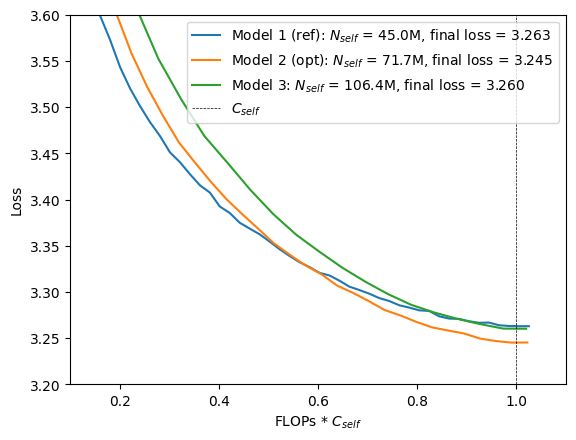
These models are summarized in Tables 1 and 2. Model 1 is the reference model and model 2 is the predicted compute-optimal model. For having models both smaller and larger than the predicted compute optimal model a third model with $N_{self} = 1.06\mathrm{e}{+8}$ parameters is added.
from article import experiment_setup

models = [m_ref, m_pred, ModelInfo(num_channels=728, num_layers=13, compute_estimator=ce)]
experiment_setup(models, c_ref=c_ref, batch_size=batch_size)
| num_channels | num_layers | num_steps | $D_{iso}$ | $N$ | $N_{cross}$ | $N_{self}$ | $C$ | $C_{cross}$ | $C_{self}$ | $\hat{C}_{self}$ | |
|---|---|---|---|---|---|---|---|---|---|---|---|
| 1 | 512 | 9 | 50000 | 2.05e+09 | 4.58e+07 | 7.86e+05 | 4.50e+07 | 5.93e+17 | 1.45e+16 | 5.78e+17 | 5.53e+17 |
| 2 | 624 | 11 | 31421 | 1.29e+09 | 7.27e+07 | 9.58e+05 | 7.17e+07 | 5.91e+17 | 1.27e+16 | 5.78e+17 | 5.54e+17 |
| 3 | 728 | 13 | 21231 | 8.70e+08 | 1.08e+08 | 1.12e+06 | 1.06e+08 | 5.89e+17 | 1.12e+16 | 5.78e+17 | 5.55e+17 |
num_channels: model dimension, num_layers: number of attention layers: $N = N_{cross} + N_{self}$: number of model parameters, $C = C_{cross} + C_{self}$: training FLOPs, $\hat{C}_{self}$: training FLOPs with $6 N_{self} D_{iso}$ approximation, $D_{iso}$: number of latent training tokens required for compute budget $N_{self}$, num_steps: number of training steps required for compute budget $N_{self}$.from article import experiment_ratios
experiment_ratios(models)
| $N_{cross} \over N$ | $C_{cross} \over C$ | ${C_{self}} \over {\hat{C}_{self}}$ | |
|---|---|---|---|
| 1 | 0.0172 | 0.0245 | 1.0455 |
| 2 | 0.0132 | 0.0216 | 1.0437 |
| 3 | 0.0104 | 0.0191 | 1.0414 |
When training these models under the same self-attention compute budget $C_{self} = C_{ref}$, we can see that the final validation loss of the compute-optimal model is actually less than that of the two other models, consistent with the prediction from the scaling law. The self-attention compute budget $C_{self}$ is indicated by a vertical dashed line.
import matplotlib.pyplot as plt

from article import plot_experiment

model_labels = ["Model 1 (ref)", "Model 2 (opt)", "Model 3"]

plot_experiment(models, model_labels, experiment_name="scaling-1")
plt.xlim(0.1, 1.1)
plt.ylim(3.2, 3.6);
Experiment 2a
This experiment trains a series of Perceiver AR models that use a UTF-8 bytes tokenizer with a vocabulary of size $262$ ($= 256 + 6$ special tokens). The prefix sequence has $m = 3584$ tokens i.e. $2048$ tokens more than in Experiment 1. The training dataset is bookcorpus.
ce = ComputeEstimator(vocab_size=262, max_seq_len=4096, num_latents=num_latents)
m_ref = ModelInfo(num_channels=512, num_layers=9, compute_estimator=ce)
models = [
    m_ref,
    ModelInfo(num_channels=584, num_layers=10, compute_estimator=ce),
    ModelInfo(num_channels=584, num_layers=9, compute_estimator=ce),
    ModelInfo(num_channels=432, num_layers=7, compute_estimator=ce),
    ModelInfo(num_channels=768, num_layers=13, compute_estimator=ce),
]

c_ref, d_ref = training_flops(ref_model=m_ref, num_steps=26144, batch_size=batch_size)

experiment_setup(models, c_ref=c_ref, batch_size=batch_size)
| num_channels | num_layers | num_steps | $D_{iso}$ | $N$ | $N_{cross}$ | $N_{self}$ | $C$ | $C_{cross}$ | $C_{self}$ | $\hat{C}_{self}$ | |
|---|---|---|---|---|---|---|---|---|---|---|---|
| 1 | 512 | 9 | 26144 | 1.07e+09 | 3.06e+07 | 1.84e+06 | 2.87e+07 | 2.16e+17 | 1.77e+16 | 1.98e+17 | 1.85e+17 |
| 2 | 584 | 10 | 18275 | 7.49e+08 | 4.35e+07 | 2.09e+06 | 4.14e+07 | 2.13e+17 | 1.55e+16 | 1.98e+17 | 1.86e+17 |
| 3 | 584 | 9 | 20298 | 8.31e+08 | 3.94e+07 | 2.09e+06 | 3.73e+07 | 2.15e+17 | 1.72e+16 | 1.98e+17 | 1.86e+17 |
| 4 | 432 | 7 | 46451 | 1.90e+09 | 1.76e+07 | 1.55e+06 | 1.60e+07 | 2.22e+17 | 2.38e+16 | 1.98e+17 | 1.83e+17 |
| 5 | 768 | 13 | 8276 | 3.39e+08 | 9.54e+07 | 2.75e+06 | 9.26e+07 | 2.09e+17 | 1.12e+16 | 1.98e+17 | 1.88e+17 |
The reference model (model 1 in Table 3) has the same number of channels and layers as the reference model in Experiment 1 but is significantly smaller because of the smaller vocabulary. Optimal model sizes are predicted with scaling laws from approaches 1 and 2:
print(f"N_opt (approach 1) = {scaling_law_1.n_opt(c_ref):.2e}")
print(f"N_opt (approach 2) = {scaling_law_2.n_opt(c_ref):.2e}")
N_opt (approach 1) = 3.90e+07
N_opt (approach 2) = 4.33e+07
Models that come close to these predictions are models 3 and 2 in Table 3 respectively. Model 4 is the smallest model in this series, model 5 the largest. The cross-attention contributions for these models are shown in Table 4. As expected, the cross-attention contribution increases because of the longer prefix sequence and smaller model sizes.
experiment_ratios(models)
| $N_{cross} \over N$ | $C_{cross} \over C$ | ${C_{self}} \over {\hat{C}_{self}}$ | |
|---|---|---|---|
| 1 | 0.0600 | 0.0822 | 1.0723 |
| 2 | 0.0481 | 0.0724 | 1.0644 |
| 3 | 0.0531 | 0.0798 | 1.0635 |
| 4 | 0.0881 | 0.1074 | 1.0820 |
| 5 | 0.0289 | 0.0536 | 1.0505 |
When training these models, the reference model is the one with the lowest loss. The predicted compute-optimal models, which are bigger, have a higher loss but are still very close to the reference model. It seems that the scaling laws overestimate the optimal model size when using a UTF-8 bytes tokenizer with a much smaller vocabulary, at least on this small scale.
model_labels = ["Model 1 (ref)", "Model 2 (opt 2)", "Model 3 (opt 1)", "Model 4", "Model 5"]

plot_experiment(models, model_labels, experiment_name="scaling-2a")
plt.xlim(0.1, 1.2)
plt.ylim(0.85, 1.0);
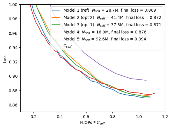
Another reason might be that the model size differences between the reference model and the predicted compute-optimal models are too small. This is supported by the higher losses of models 4 and 5. In [1] section 3.2, the authors also used "a diverse enough set of model sizes" in order to observe a clear minimum in the IsoFLOPs profiles.
Experiment 2b
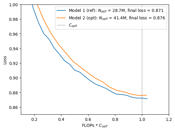
Another reason for the observed overestimate of compute-optimal model sizes in Experiment 2a could be the longer prefix sequence compared to Experiment 1. To verify that, I used a shorter prefix sequence of length $m = 1536$ for models 1 and 2.
ce = ComputeEstimator(vocab_size=262, max_seq_len=2048, num_latents=num_latents)
m_ref = ModelInfo(num_channels=512, num_layers=9, compute_estimator=ce)
models = [m_ref, ModelInfo(num_channels=584, num_layers=10, compute_estimator=ce)]

c_ref, d_ref = training_flops(ref_model=m_ref, num_steps=26144, batch_size=batch_size)

experiment_setup(models, c_ref=c_ref, batch_size=batch_size)
| num_channels | num_layers | num_steps | $D_{iso}$ | $N$ | $N_{cross}$ | $N_{self}$ | $C$ | $C_{cross}$ | $C_{self}$ | $\hat{C}_{self}$ | |
|---|---|---|---|---|---|---|---|---|---|---|---|
| 1 | 512 | 9 | 26144 | 1.07e+09 | 2.95e+07 | 7.86e+05 | 2.87e+07 | 2.06e+17 | 7.60e+15 | 1.98e+17 | 1.85e+17 |
| 2 | 584 | 10 | 18275 | 7.49e+08 | 4.23e+07 | 8.97e+05 | 4.14e+07 | 2.05e+17 | 6.63e+15 | 1.98e+17 | 1.86e+17 |
Training these two models results again in a higher loss for the predicted compute-optimal model i.e. the scaling laws also overestimate the optimal model size here. This suggest that the smaller vocabulary rather than a longer prefix sequence is the reason why the experimental results do not match the prediction.
model_labels = ["Model 1 (ref)", "Model 2 (opt)"]

plot_experiment(models, model_labels, experiment_name="scaling-2b")
plt.xlim(0.1, 1.2)
plt.ylim(0.85, 1.0);
Conclusion
Scaling law predictions match the experimental results when the same tokenizer as in the Chinchilla paper [1] is used (a SentencePiece tokenizer) but they seem to overestimate the optimal model size $N_{opt}$ when using a UTF-8 bytes tokenizer which uses a much smaller vocabulary. These are results from training Perceiver AR models on a small scale. It needs to be investigated if a similar trend can be observed on larger scale too.
The scaling laws can only be applied to the self-attention part of Perceiver AR since they have been derived from training data of decoder-only transformers. The small cross-attention contribution to the overall compute must be taken into account separately when allocating a compute budget. The direct impact of prefix cross-attention on model performance, under a given compute budget, was not analyzed here and requires further experiments.
References
[1] J. Hoffmann, S. Borgeaud, A. Mensch, E. Buchatskaya, T. Cai, E. Rutherford, D. de Las Casas, L. A. Hendricks, J. Welbl, A. Clark, et al. Training compute-optimal large language models. arXiv preprint arXiv:2203.15556, 2022.
[2] C. Hawthorne, A. Jaegle, C. Cangea, S. Borgeaud, C. Nash, M. Malinowski, S. Dieleman, O. Vinyals, M. Botvinick, I. Simon et al. General-purpose, long-context autoregressive modeling with Perceiver AR. arXiv preprint arXiv:2202.07765, 2022.
[3] J. Kaplan, S. McCandlish, T. Henighan, T. B. Brown, B. Chess, R. Child, S. Gray, A. Radford, J. Wu, and D. Amodei. Scaling laws for neural language models. arXiv preprint arXiv:2001.08361, 2020.
Comments